We have interactivity! Check out the qualifying delta plot shown below.
Qualifying teammate battles seem to be of great interest to the current F1 community. While I’m a firm believer that Sundays are much more important than Saturdays, I will accept that qualifying has a great impact on a race, especially when you consider how hard it is to overtake with the latest generation F1 cars.
Analysis
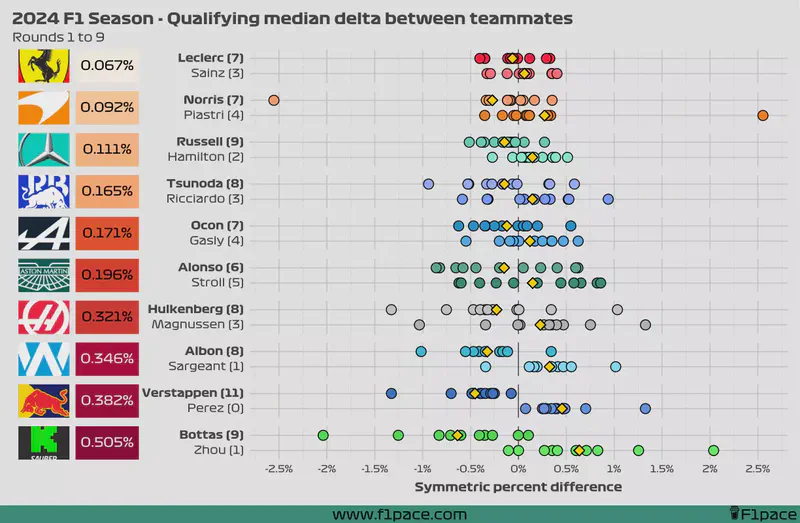
Overall qualifying median delta
This interactive chart is better visualized on a computer.
If you’re on a mobile device, tap and hold the chart to reveal the toolbar on the left. This toolbar enables zooming and scrolling. Hover over the data points to see a tooltip with additional information. On mobile devices you may need to click and hold the points to display the tooltip.
I don’t have much to say today. I’m pretty tired to be honest. I’m not sure it’s worth it to continue doing this. Anyways, I’ve switched the analysis to use the median instead of the mean just to avoid crazy outliers in rainy sessions. The median is more resistant to outliers so even if we have an extreme session here and there, it should stay true to reality.
Cumulative qualifying median delta
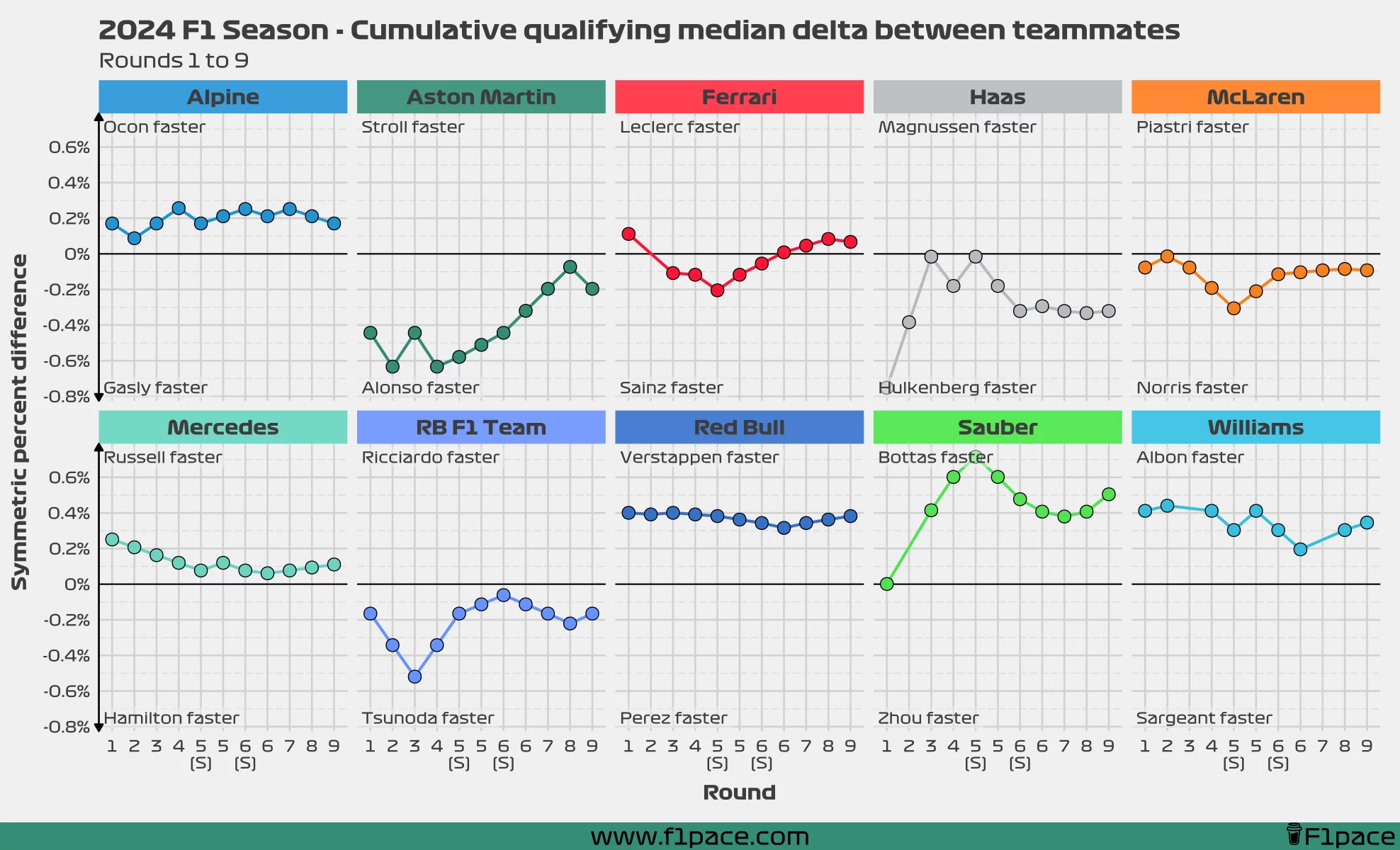
We can also visualize the cumulative difference between teammates by using a rolling average. This method involves adding each race’s data as the season progresses and then computing an average. The goal is to identify trends over time. This trend shows if a driver is getting closer, farther or at the same distance to his teammate.
Since I’m only interested in a 1v1 analysis between teammates, I decided to keep only the official race drivers for this analysis. This means that I removed the data from Oliver Bearman since I’m only interested in the Leclerc vs Sainz battle for the Ferrari team.
Methodology
I calculated the delta between teammates by using the symmetrical percent difference. To find out why I did this, check the “issues” section after the analysis.
For each race and for the highest qualifying session that both drivers from the same team reached I calculated the symmetric percent difference. Negative values mean that a driver was faster than his teammate, while positive values mean that the driver was slower than his teammate. A difference of 0% means that both drivers were just as fast.
I calculated the values for each race for each team and plotted them as individual data points in the chart. I then calculated the median of these values for the season (so far) and displayed it the left side of the plot, next to the team logo. Smaller overall values represent that both teammates were more evenly matched during quali, while larger overall values show a greater gap between teammates.
Additionally, on the left-hand side of the chart next to the driver’s name, I also added the number of times a particular driver has been faster than his teammate in quali.
Finally, I added a gold-coloured diamond to show the median gap between teammates. This number will be equal to the overall value displayed on the left side of the plot, next to the team logo.
For the cumulative plot, I gathered data from each race and calculated a rolling median For example, for race 5, I used the qualifying delta from the first five races to compute the median As more races occur, additional data is incorporated into the rolling median, resulting in a more stable and accurate trend.
Issues!
One of the main issues when gathering data from multiple races is that the deltas will change depending on the length of each track. A delta of 0.1 seconds in a short track (say, 1:05 per lap) will be greater than a delta of 0.1 seconds in a long track such as Spa (~ 1:45).
One way we can standardize the data is by converting the deltas to percentages, but there is one big issue with this. The traditional way of calculating a percent difference is with the following formula:
$$ Percent\ difference = 100\times\frac{value1-value2}{value2} $$
The main problem is that this value is not symmetrical. This means that if I reverse the order of value 1 and value 2, the final percent difference will be different.
$$ Percent\ difference = 100\times\frac{80-90}{90}=-11.11\% $$ $$ Percent\ difference = 100\times\frac{90-80}{80}=12.5\% $$
You can see that the percentages are not reversible, even though in both cases we’ve changed the original value by 10 units.
One way we can solve this problem is by using the symmetric percent difference, which is calculated by using the following formula:
$$ Symmetric\ percent\ difference = 100\times\frac{value1-value2}{(value1+value2)/2} $$ This formula is reversible, meaning that regardless of the order of the values, we will get the same result. Because of this, I decided to use the symmetric percent difference formula as the basis for the analysis.